 next to the formula bar. Choose Financial and then PMT
Loans
Most people at some point will have a car loan, student loan and/or a home mortgage. We are working in particular with fixed rate loans. With a fixed rate loan, you pay the same amount monthly (to be determined using the PMT function in Excel) for the entire duration of the loan. For example, a loan for $10,000 to purchase a car which is paid back over 5-years at an annual interest rate of 6%. To see how the loan is paid back, you will learn how to create an amortization table. Ultimately, you should understand a little how loans behave, in particular, how the principal goes down very slowly at first and how especially over long periods of time, total payments can be 2 or even 3 times the total principal (the amount of the loan).
We will create an example of an amortization table which assumes a 6% interest rate, 5 year duration and 10,000 loan amount. You will always be given these three amounts which you will need to complete a loan problem. The only minor concern with this spreadsheet is that is doesn't round to two decimal places (so it balances to zero which is nice). So technically, we are using fractional cents which doesn't make sense in the "real" world. You should use the rounding function in Excel but we won't worry about it as part of this class.The follow steps show you how to construct an amortization table . It is important to do the steps in order.
1. Fill-in headings across in the first row (see below). (Type "Month in cell A1, Beginning Balance in cell B1, etc…)Amortization Table
Month |
Beg Balance |
Payment |
Interest |
Principal |
End Balance |
0 |
|||||
1 |
|||||
2 |
2. Fill-in the total number of months going down (type in 0 and 1 then select both numbers and then fill down by dragging). For this example, you should fill down to 60. You need this column established to fill down the formulas you put in cells B3, C3, D3, E3 and F3.
3. Type in loan amount in cell F2. This is the only cell (besides the headings and the months) that doesn't have a formula. For this example, fill in 10000 (do not include the comma when you type it in).4. Fill-in the following formulas in cells B3, C3, D3, E3 and F3
a. In cell B3 type "=F2"
to carry the ending balance of the previous month to the beginning balance of
the next month.
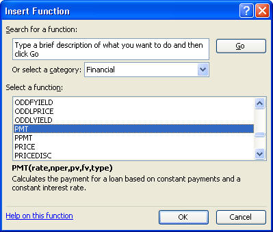
b. In cell C3 calculating the monthly payment using the
PMT function in Excel as shown below.
Click on
Enter the Rate which is .06/12 (it is always the
annual interest rate is divided by 12).
Enter the
number of payments, Nper, which is 60 or 12*5.
Enter the
loan amount, Pv, as a negative number which is -10000 for this example.
Leave Fv and
Type blank (we just use the defaults)
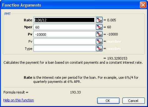
Then hit ok to enter the result in the cell.
d. Calculate the amount of interest
owed that month which is the balance times the interest rate divided by 12.
In cell D3 type "=B3*.06/12".
The interest is
the money that the bank keeps or the cost of getting a loan.
e. Calculate the principal for that month by
subtracting the interest owed from the payment. In cell E3 type
"=C3-D3".
This is the amount that actually reduces the beginning balance.
f. To get the balance at the end of the month,
in cell F3 type "=B3-E3".
6. Fill down B3 through F3 (which has already been selected in the step above) by double clicking on the fill down box.
7. Verify that the ending balance in the last line is zero!You have just created an amortization table. To determine how much you paid to borrow 10,000, sum the interest column by clicking on the first empty cell at the bottom of the interest column. Click on the AutoSum button and hit enter. For this example, you paid $1599.68 to borrow $10,000. The total amount you paid out is $11,599.68 (the sum of the payment column). If you total the principal column, you will get the amount of the loan, $10,000.